StatCrunch Featured Data Sets
In August, 2018, Pearson posted a wide variety of featured data sets that you can use to illustrate a variety of statistical concepts in your class. Each data set on this site has a thorough description of the data and provides a source along with descriptions of each variable.
I would like to focus on the “California Home Prices, 2009” data set. This particular data set is interesting because it represents a variety of variables on homes sold in San Luis Obispo county during the financial crisis that started in August, 2008 (including sale type such as regular, foreclosure, or short sale). Many of our students would have been between 8 and 10 years old during this very scary time in our country’s financial history, so I think students would benefit from a brief discussion of what happened during the financial crisis – especially as it pertains to “easy” credit being extended to folks who wanted to purchase homes. Some of the mortgages people secured to buy homes were interest only and others were adjustable rate mortgages. In an adjustable rate mortgage, the interest rate on the loan may increase as the interest rate the mortgage is based on increases (such as the federal funds rate). One outcome of the crisis was massive decline in home prices which caused many folks to have their home prices plummet below the amount they owed on the home. As a result, homeowners were either foreclosed upon or sold their home for less than they owed (short-sale).
The Guidelines for Assessment and Instruction in Statistics Education (GAISE) report released in 2016 provides a variety of recommendations while teaching Introductory Statistics. One such recommendation is to “give students experience with multivariable thinking.” This data set provides a relatively easy way to address this recommendation.
Begin by drawing a scatter diagram of “Price” against “SQFT” treating SQFT (square footage) as the explanatory variable.
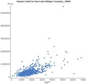
Notice the positive association between the two variables. However, there is an observation that is potentially an outlier and/or influential. Use your mouse to draw a square around the observation. After doing this the observation changes color to magenta. Hit the down arrow on the spreadsheet to see which house this value corresponds to. It is a 5060 square foot home that sold for $5,499,000 and is located in Arroyo Grande.
Notice that there are three types of sales reported in this data set (Foreclosure, Regular, and Short Sale). You might ask students to research what each of these sales types represent. Then, ask students to draw a scatter diagram by Status (use the “Group by:” drop-down menu in the Scatter Plot dialogue box). This way, we are introducing a qualitative variable to the analysis and may be able to visualize the role status plays in any association between square footage and price. What do you see in the graph?
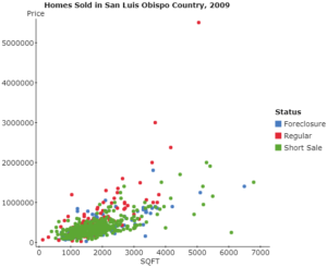
Based on the graph, it looks like status plays a role in the association between square footage and sales price. So, now students could find the linear correlation between the two variables by status (again, use the “Group by:” in the dialogue box). All three status sales have roughly the same correlation.

Or, we could find the least-squares regression between square footage and sales price (treating square footage as the explanatory variable).
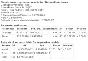
In the screen shot above, the least-squares regression between square footage, x, and sales price, y, is
![]() Status = Foreclosure
Status = Foreclosure
The least-squares regressions for the other status sales is:
![]() Status = Regular
Status = Regular
![]() Status = Short Sale
Status = Short Sale
Students should interpret the slope of each regression as follows: When the status is foreclosure, if the square footage increases by 1 square foot, the expected sale price increases by $236. The obvious thing to note is that the slope of regular sales is much higher than the other two. What does this suggest? Distressed sales make the sales price increase much less, on average, as square footage increases. Ask students if it makes sense to interpret the intercept. The answer is that it does not because a home with 0 square feet does not make sense (and 0 square feet is outside the scope of the model).
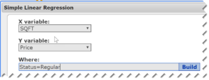
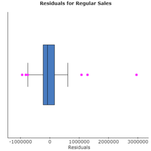
Finally, it is worthwhile to focus on the regular status homes (due to the potential outlier/influential observation). To determine if the observation is an outlier, save the residuals when doing a regression. Then, draw a residual plot and also a boxplot of the residuals.
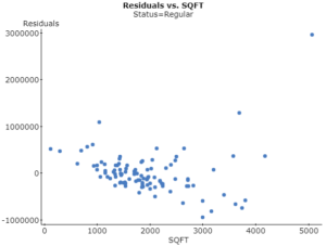
The residual plot does not show any obvious pattern (other than the potential outlier), so a linear model is appropriate in describing the association between square footage and price. In the boxplot, notice there are a number of outliers (surprising given the residual plot). The largest residual corresponds to the 5060 square foot home in Arroyo Grande mentioned earlier.
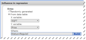
We also want to know if Arroyo Grande observation is influential. While advanced methods for identifying influential observations exist, at the introductory level, I recommend a simple graphical test using StatCrunch’s “Influential Observation” applet. To use this applet, select Applet > Regression > Influence in StatCrunch. Fill in the dialogue box as shown below. Click Compute!.
Use your mouse to draw a square around the alleged influential observation (in the upper-right portion of the scatter diagram. The observation becomes a square and two regression lines appear – one is the regression line that includes the alleged influential point; one is the regression line without the point.
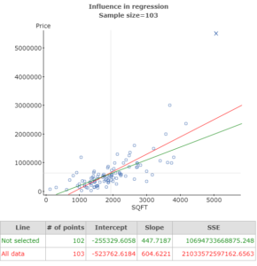
Notice the slope without the observation (green line) in Arroyo Grande is $447.7/square foot and the slope with the observation (red line) is $604.6/square foot – a 26% decrease. It would appear this one observation is influential. So, while the slope of the least-squares regression line for regular sales is still much higher than it is for other sales (Foreclosure or Short Sale), the difference is not as extreme as it would appear from our original analysis.
This StatCrunch data set provides lots of opportunities for students to explore. Most important, is that students are exposed to some multivariable thinking. Perhaps students could explore the role the other variables (location, number of bedrooms, number of bathrooms) plays in the selling price.
Recent Posts
- Artificial Intelligence in Statistics 7e 12/19/2024
- Recent Webinar 03/19/2024
- Article on Alternative Grading 12/12/2023
- Article on DEVELOPING A STATISTICS COURSE FOR STUDENTS IN NON-QUANTITATIVE FIELDS 11/10/2023
- Article on Florence Nightingale 09/26/2023
Categories
- Classroom Strategy (10)
- Data Set (2)
- Research Article (3)
- Statistics Articles (4)
- Textbooks (3)
- Uncategorized (7)
